Dimensionality reduction of neural data

Recording capabilities in neuroscience are increasing fast. Whereas for decades the norm was to record activity from one or a few neurons, over the last decade this has rapidly increased to simultaneous recordings from dozens, hundreds and recently even thousands of neurons. Alongside this increase in recording capabilities, there has been a shift in focus in analysis techniques. Where analyses previously focused on activity from single neurons there is now a lot of attention for population activity (the activity of many neurons). The central question here is whether there is structure in the neural activity that is shared among multiple neurons. A nice way to understand the essence of population analyses is to consider the information contained in a photograph. This photograph has many pixels that all convey some independent information. However, there is also some representation that is shared among the pixels, i.e. the information is correlated across subsets of pixels. Similarly, individual neurons can (and do) convey independent information, but some part of the information they represent is shared among many neurons. Some have provided evidence that this population activity constitutes a fundamental and stable building block of brain activity and behaviour, that it is the fundamental unit of brain activity.

To find this shared information representation, it is useful to apply dimensionality reduction techniques. These techniques find the (low-dimensional) representation that is shared amongst the (high-dimensional) activity of many individual neurons. In this post, I will discuss some of the core concepts of dimensionality reduction and apply principal component analysis (PCA), one of the most popular dimensionality reduction techniques.

Code availability

The code to reproduce these analyses is available as a jupyter notebook on my github page.

Overview of the data

I will very briefly describe the data so that we can interpret what our results mean. The data used for this post is one example recording from the dataset described in my thesis and this recent article (which discusses a different form of dimensionality reduction: Hidden Markov Models). This recording is from the primary visual cortex (V1) using 16-contact linear electrodes (there were 16 electrode contacts) with which we recorded neural activity. In V1, neurons respond to visual stimuli when they are presented in a small part of the visual field, their receptive field (RF).

The paradigm

On each trial, three stimuli (coloured gratings) were presented. Although they were exactly the same on each trial, it varied which of the stimuli was relevant (and thus to which stimulus attention should be directed). The relevant stimulus was indicated by a central square that matched the colour of one of the stimuli. This stimulus needed to be monitored for a change in luminance (dimming), which could occur first, second or third in the dimming sequence.

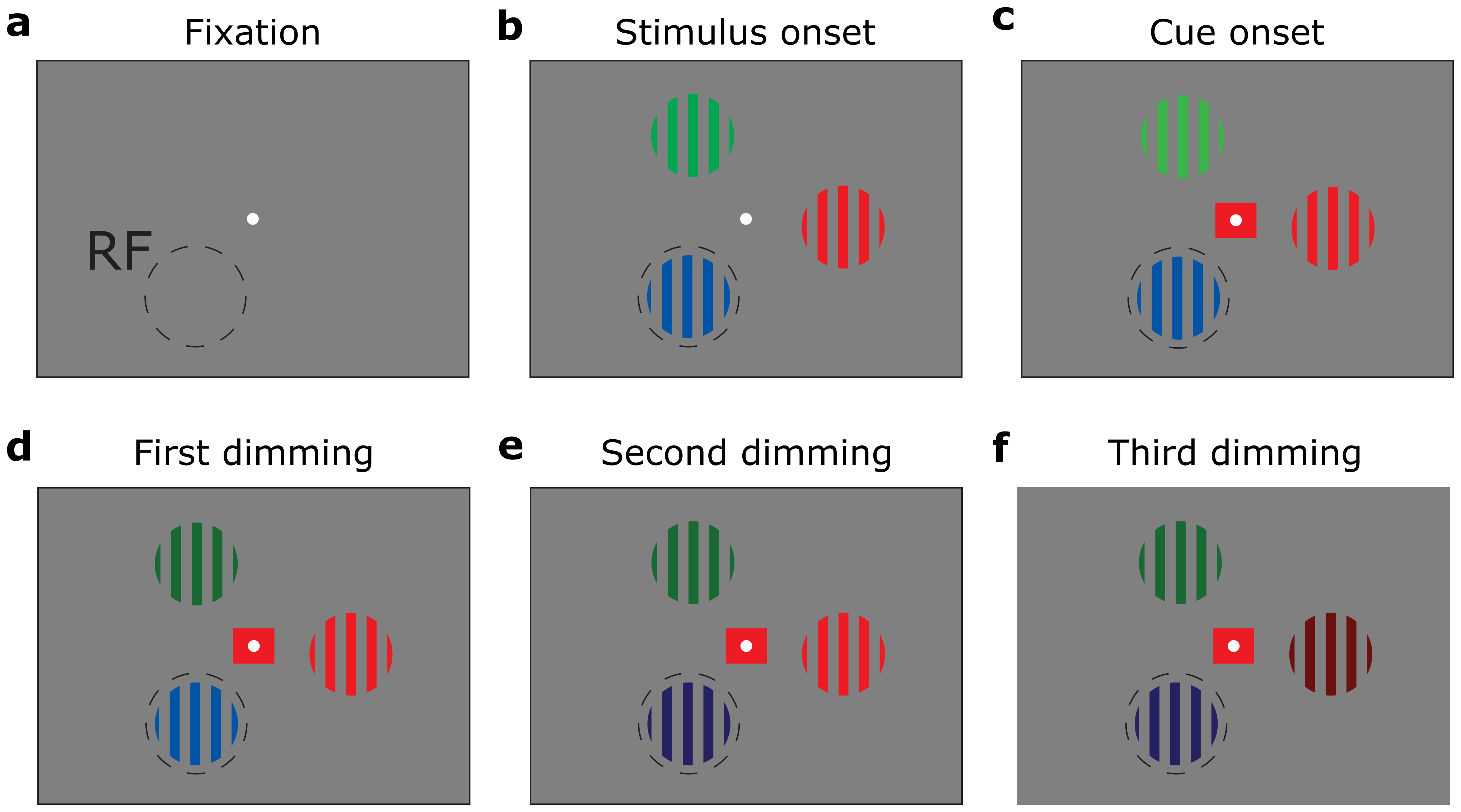
Paradigm, example trial sequence. The red grating is behaviourally relevant on this trial and should be monitored for a change in luminance (dimming)

Crucially, the cue, indicating which of the 3 stimuli to attend to, was presented after the stimuli. This means that the cognitive “attention” signal only originates a few 100 ms after the onset of the cue.

Visual response

Lets have a look at the data, starting with the trial-averaged activity aligned to stimulus onset. As you can see, there is a reliable stimulus-induced response on most of the channels.

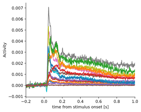
Visual response for each individual channel

Attentional effects

When attention is directed towards the RF, neurons generally increase their activity. As the neurons in V1 only respond to stimuli presented inside their RF, attention modulates this activity only when when attention is directed towards the stimulus inside their RF. From the perspective of these neurons, the two conditions where attention is directed away from the RF (to the other two stimuli) are not different. This will be important to keep in mind for the interpretation of the results below.

This plot shows the trial and channel-averaged activity for each of the three attention conditions. When attention is directed towards the RF, activity increases after onset of the cue relative to the other two conditions.

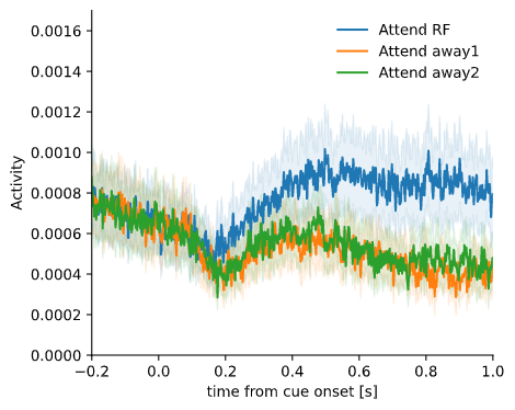
Attentional modulation of activity, averaged across channels

Dimensionality reduction

Now that we have a basic understanding of the activity present in this data, I will discuss eigendecomposition and principal component analysis (PCA).

The goal of these analyses is to find a low-dimensional representation that captures much of the variance (information) of the original high-dimensional data. In this case, we have a recording of 16 channels, so our data is 16-dimensional.

To some degree, neural activity covaries between the channels within one area, i.e. the trial-to-trial variability in neural responses is shared across channels. This covariance reveals structure in the data; we assume that:

• directions of large variation represent signal (interesting features in the data)
• directions of small variation represent noise

The goal of PCA is to find these directions of maximal covariance. Once identified, we can project the data onto these directions and represent the data in a lower dimensional space. The directions of maximal variance in the data are the directions indicated by the eigenvectors of the covariance matrix.

How do we perform PCA? There are three main steps:

1. Subtract the mean
2. Calculate the eigenvectors of the covariance matrix, sorted by the corresponding eigenvalue
3. Project the data onto the new basis

Covariance matrix

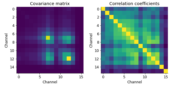
Lets first have a look at the covariance and correlation coefficients. Having averaged the activity within a particular time window, our data are matrices of size 746 trials \(\times\) 16 channels. Thus, we have a tall matrix \(X\) of size 746 \(\times\) 16.

The covariance matrix is obtained by \(X^{T}X\) (np.cov also normalises by \(n-1\) corresponding to the degrees of freedom, where \(n\) is the number of samples, i.e. trials) and results in a matrix of size 16 \(\times\) 16, with an entry on both axes for each channel. Values in this matrix indicate whether activity between channel pairs covaries across trials (with unit: activity\(^{2}\)). The covariance matrix \(X^{T}X\) encodes all the linear interactions among the variables/columns of X.

I also plotted the correlation coefficients, which is the normalised version of the covariance matrix (normalised by \(\sqrt{var(x_{1})var(x_{2})}\) ), scaling the covariance values between -1 and 1. This sometimes gives a little more insight into which channels/features covary.

# calculate covariance and correlation coefficient matrix
cov_matrix = np.cov(plotdata['V1'], bias=True, rowvar=False)
corr_matrix = np.corrcoef(plotdata['V1'], rowvar=False)

An example using 2 channels

We will first run the entire procedure across a subset of the data, the activity from 2 channels. Here, our data matrix data_mat is thus 746 \(\times\) 2.

idx_unit = [6,7] # select units to plot 

# extract data
data_mat = plotdata['V1'][:,idx_unit]

# mean center
data_mat = data_mat - np.mean(data_mat, axis=0)[np.newaxis,:]

# compute covariance matrix
cov_matrix = np.cov(data_mat, bias=True, rowvar=False)

# eigendecomposition
evals, evectors = np.linalg.eigh(cov_matrix)

# sort eigenvalues/vectors by eigenvalue
index = np.flip(np.argsort(evals))
evals = evals[index]
evectors = evectors[:, index]

# project data onto orthonormal basis
data_proj = data_mat@evectors

From left to right we see:

• (panel 1) the covariance matrix for this 2 \(\times\) 2 case.
• (panel 2) the activity on each of these two channels (each marker is a trial) and the eigenvectors plotted on top. It is clear from this plot that the activity on these two channels covaries strongly: when there is high activity on one channel, it is likely there is high activity on the other channel.
• (panel 3) the “Scree plot” with the eigenvalues. The value of the eigenvalue is directly related to the magnitude of the variability in the direction of its corresponding eigenvector.
• (panel 4) the data projected on the eigenvectors (imagine that the eigenvectors in panel 2 form the new axes for the data). Rather than channels, we now speak of components in the data.

Some key characteristics of eigendecomposition/PCA

We can verify a few of the key properties of eigendecomposition/PCA in order to get a better understanding of what is happening here.

Some key properties of PCA:

1. Eigenvectors are orthogonal
2. As a result, the components (columns) of the projected data are uncorrelated
3. The variance of each component of the projected data is equal to its corresponding eigenvalue

1. Eigenvectors are orthogonal

One of the most important characteristics of orthogonal vectors is that their dot product is zero. As these eigenvectors are also unit length, the dot product of one eigenvector with itself is one. Therefore, matrix multiplication between eigenvectors should result in the identity matrix.

print(np.round(evectors.T@evectors))

[[ 1. -0.]
 [-0.  1.]]

2. The components are uncorrelated

Testing the correlation between the projected data (components) shows that the correlation between components is zero (within machine precision).

corr_matrix = np.corrcoef(data_proj, rowvar=False)
print(corr_matrix)

[[ 1.00000000e+00 -4.05554456e-16]
 [-4.05554456e-16  1.00000000e+00]]

3. The variance of each component is equal to its corresponding eigenvalue

The variance of the components is equal to their corresponding eigenvalue.

print(np.var(data_proj, axis=0))
print(evals)

[1.41607049 0.07771349]
[1.41607049 0.07771349]

Achieve the same result using PCA

OK! Now that we’ve gone through these procedures step-by-step, we’ll do it all again but quicker. We can replicate this analysis by using the principal component analysis (PCA) function of the sklearn.decomposition package in only a few lines of code.

pca = PCA(n_components=2).fit(data_mat)
evectors = pca.components_.T # transpose evectors
evals = pca.explained_variance_
cov_matrix = pca.get_covariance()
data_proj = pca.transform(data_mat)

Expand to higher dimensions

Next, we can do the same for all available channels. In our case we have 16 channels, so we have a 16-dimensional space that we can project to a few principal components. Then, after the projection, we can have a look at whether any of these dimensions explain variance related to any of the task parameters, for instance the attention condition.

# extract data
data_mat = plotdata['V1']

# mean center
data_mat = data_mat - np.mean(data_mat, axis=0)[np.newaxis,:]

# apply PCA
pca = PCA(n_components=16).fit(data_mat)

# get components/eigenvectors and eigenvalues
evectors = pca.components_.T # transpose evectors
evals = pca.explained_variance_

cov_matrix = pca.get_covariance()

# project data, get scores
data_proj = pca.transform(data_mat)

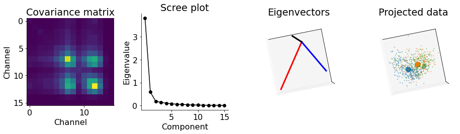
From left to right we see:

• (panel 1) the covariance matrix.
• (panel 2) the “Scree plot” with the eigenvalues.
• (panel 3) the first three components.
• (panel 4) the data (and their means) projected onto the eigenvectors for the first three components (three axes) for the three attention conditions (blue is attend RF).

From this we can conclude that there is one component that explains (by far) the most variance in the data. Next, we separate the data according to the attention conditions. Although it is not immediately obvious that information relevant to attention is encoded along these directions, as the center of mass of the three clusters seems to be in a slightly different location, there might be something more to explore there.

PCA over time

Alright, now for the exciting bit! We do not have to pick an arbitrary time window, average the activity in this window and then apply PCA on this activity. We can apply PCA to all the data (over channels, trials and time) at once.

To start off with, we have all our activity aligned to the onset of the cue in the variable attention_activity of size (num_channel, num_trial, num_time).

print(np.shape(attention_activity))

(16, 746, 1221)

We can reshape this 3D matrix into a 2D matrix.

pca_activity = np.reshape(attention_activity, (np.shape(idx_unit)[0],-1))
pca_activity = pca_activity.T

print(np.shape(pca_activity))

(910866, 16)

and apply PCA across this entire matrix.

# apply PCA
pca = PCA(n_components=3).fit(pca_activity)
evectors = pca.components_.T
evals = pca.explained_variance_

# project onto eigenvectors
data_proj = pca.transform(pca_activity)

# reshape (back) to (component x trial x time)
data_proj = np.reshape(data_proj.T, (3, -1, np.shape(attention_activity)[2]))

# get explained variance
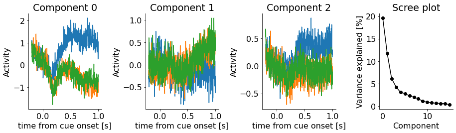
evals_percentage = pca.explained_variance_

When we then sort the data according to the attention conditions, we see that the first component distinguishes between these conditions! Thus, the component that explains the most variance is the direction in PCA space that is relevant for cognitive (internal) functions such as attention.

3D visualisation

animation over time

A nice way to visualise these results is to plot the progression of activity in 3D over time. For this I use the custom pyplotj.animj module.

Here we clearly see that a few hundred milliseconds after onset of the cue, the activity in the attend RF condition occupies a different location in PCA space.

Conclusion

Dimensionality reduction and PCA are great ways to explore, summarise and visualise high-dimensional data. I hope this post has been helpful. Have fun applying it to your own data!

Setup & notes

Environment setup & installation of packages

conda create -n dim-reduction-demo python=3.8 numpy scikit-learn pandas matplotlib scipy
conda activate dim-reduction-demo

Loading packages

# import packages
import sys
from matplotlib import pyplot as plt
from matplotlib import rcParams 
from mpl_toolkits.mplot3d import axes3d
import matplotlib.animation as animation
from IPython.display import HTML

import numpy as np
import numpy.matlib
import os
from sklearn.decomposition import PCA 

# custom packages/modules
from pyplotj import animj
from neuroimport import matlabimport

Importing/Loading data

The data are in the MATLAB format (.mat files) and need to be imported into python. For this I use the scipy library (scipy.io.loadmat) and the custom module neuroimport.matlabimport.