Gain variability

Spike count distributions have historically been modeled as a Poisson process. In a Poisson process, the events of interest (in this case spikes) occur at random within a given time interval. The Poisson probability mass function lets you obtain the probability of an event occurring within a given time or space interval exactly \(x\) times if on average the event occurs \(\lambda\) times within that interval. It reflects the number of times (count) of occurrences of random events (in this case spikes) in a fixed interval (see here and here for a detailed discussion).

A key property of the Poisson distribution is that the variance is equal to the mean. However, spiking data often displays super-Poisson variability (greater variance than the mean). To accomodate this, Goris et al., proposed to modify the Poisson distribution so that the additional variance, termed gain variability, is captured by a Gamma distribution. Mixing a Poisson and Gamma distribution results in a negative binomial distribution (as discussed here, and here). The negative binomial distribution has a mean \(\lambda\) and dispersion/rate parameter \(\beta\) (inverse of scale), and its variance is defined as \(\lambda + \beta \lambda^{2}\). As this value is larger than \(\lambda\), the negative binomial distribution is always overdispersed.

I created a toolbox to model spike count distributions using a negative binomial distribution. The code can be found on my github page. I’ve included a couple of examples on how to use this package.

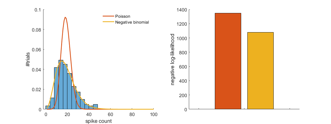
Fitting a Poisson and negative binomial distribution to across-trial spike count data